Deep Q-Learning
Slides rl-3.pdf
Briefing
Last week we implemented Q-Learning, which uses a lookup table, defining the Q-Value for every (state,action) pair. This becomes a map \[(\text{state},\text{action}) \mapsto \text{value}\] We can also read it as a map from state to a list of action/Q-value pairs \[\text{state} \mapsto \{ (\text{action}_i,\text{value}_i) \}\] or a map \[\text{state} \mapsto (\text{action},\text{value})\] where the action and value are found by taking the maximum in the row corresponding to the given state. Which formulation we use may depend on the update algorithm we choose.
In Deep Q-Learning we replace the lookup table with a deep neural network. In our formulation below, we shall see it as a map \[\text{state} \mapsto \{ (\text{action}_i,\text{value}_i) \}\] The neural network (or any regression or classification model in general) takes an input and predicts the corresponding output. During training the weights or parameters of the model are tuned to minimise the error on a given training set.
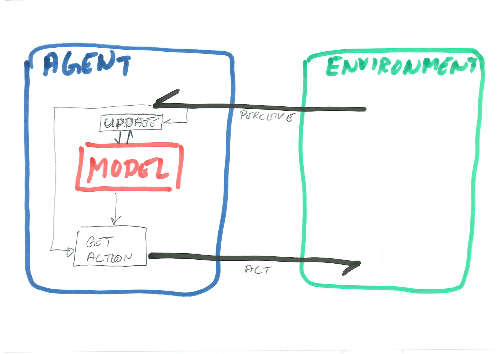
Hence, in the RL Agent in the diagram, the model is a neural network, and the get action operation is simply an evaluation of the network. The tricky part is the update method. Unlike the first textbook demonstrations of machine learning, we cannot pregenerate a training set and train once and for all, because the set of bad solutions is far too large. Instead, we need to use exploration strategies similar hill climbing, so that once we find a half-good state, we explore the neighbourhood for better states.
The tutorial gives only one approach to network update. As is so often the case in machine learning and artificial intelligence, it is far from obvious what will be the best solution in any given case.
It should be noted that Deep Q-Learning is primarily designed for very large, and typically continuous, state spaces. Applying it here on the frozen lake is merely an illustration. It is a useful illustration because we can validate the solution either manuall or by comparison with regular Q-Learning.
The update method
In this session we assume an online algorithm, where we alternate between taking actions to collect experiences and training the network on a minibatch of buffered experiences. The buffer is called replay memory. The pseudo-code can look like this.
initialize replay memory D
initialize action-value function Q with random weights

repeat
   observe initial state s
   repeat
      select an action a
         with probability ε select a random action
         otherwise select a = argmax[a’] Q(s,a’)
      carry out action a

      observe reward r and new state s’
      store experience <s, a, r, s’> in replay memory D

      sample random transitions <ss, aa, rr, ss’> from replay memory D
      calculate target for each minibatch transition
         if ss’ is terminal state then tt = rr
         otherwise tt = rr + γmaxa’Q(ss’, aa’)
      train the Q network using (tt - Q(ss, aa))^2 as loss

      s = s'
   until terminated
Note the three main steps of the inner loop. First we select an epsilon-greedy action. Then we make the move and record the result in replay memory. Then we run a random batch from replay memory to improve the training. (Finally we update the state.)
Caveats This is a very simple version of the algorithm, even if it illustrates the main points. If you seek other sources you will probably find that.
- Two networks are used; one for the greedy-epsilon selection and another which is trained. Periodically the weights are copied from the latter to the former. This improves stability.
- The replay memory is not just a simple buffer holding the last \(n\) experiences. Instead experiences are selected according to multiple criteria, keeping typically some particularly significant experiences as well as some of the most recent.
However, we have enough on our plate today, and these caveats should be left for later.
Exercise
Task 1 - Tensorflow/Keras
We will start today with getting used to tensorflow/keras, you can also adapt the exercises to pytorch or similar if prefered (but code-examples will be given in tensorflow).
First, install tensorflow:
We will only be using the Keras API, you can find the documentation here
Verify in python with:
Part A - Perceptron
We can make a single perceptron with keras like this:
from tensorflow import keras
from tensorflow.python.keras.layers import Dense

model = keras.Sequential([
  Dense(units=1, input_dim=1)
])
and do a forward propagation with:
Furthermore, we can get and set the current weights with:
# Get weights
w1, b1 = model.layers[0].get_weights()
print( w1 )
print( b1 )

w1[0,0] = 1

# Set weights (TODO: replace w1 and b1)
model.layers[0].set_weights( [ w1, b1 ] )
Tasks/Questions
- Test out different values for the weight
w1and biasb1 - How do you forward-propogate multiple values at once?
- Can you plot the graph for some range of inputs?
Task 2 - Q-Values from an ANN
We still want to work with Q-values, meaning that we would like some value for all possible actions as output from our neural network. Our FrozenLake environment has 4 possible actions, and we already know the q-values for all possible states, making it easy to fit a neural network.
Part A - Creating a network
The following code will create a neural network that inputs a state (one value) and outputs 4 values (one for each action), it will also assume 16 possible states (0-15):
import numpy as np
import tensorflow as tf
from tensorflow import keras
from tensorflow.python.keras.layers import Dense

x_data = np.linspace(0, 15, 16)
normalizer = keras.layers.Normalization(input_shape=[1,], axis=None)
normalizer.adapt(np.array(x_data))

model = keras.Sequential([
	 normalizer,
	 Dense(64, activation='relu'),
	 Dense(64, activation='relu'),
	 Dense(4)
])

model.compile(
    optimizer=tf.optimizers.Adam(learning_rate=0.001),
	  loss='mse'
)
Answer the following:
- What does the
x_datalook like (data type, contents, structure)? This will be used as network input, that is, each element should be a state. - What is the design (structure) of this neural network? Look primarily on the lined defining
model.
The normalizer (which is defined after x_data) scales the input so that all features have the same magnitude.
The model.compile statement defines the optimiser algorithm (tuning the weights) and the loss function (defining the cost of current errors).
Part B - Training
As we already have Q-Values, let us train the network on the data:
y_data = np.array([
	[0.54, 0.53, 0.53, 0.52],
	[0.34, 0.33, 0.32, 0.50],
	[0.44, 0.43, 0.42, 0.47],
	[0.31, 0.31, 0.30, 0.46],
	[0.56, 0.38, 0.37, 0.36],
	[0., 0., 0., 0.],
	[0.36, 0.2, 0.36, 0.16],
	[0., 0., 0., 0.],
	[0.38, 0.41, 0.40, 0.59],
	[0.44, 0.64, 0.45, 0.40],
	[0.62, 0.50, 0.40, 0.33],
	[0., 0., 0., 0.],
	[0., 0., 0., 0.],
	[0.46, 0.53, 0.74, 0.50],
	[0.73, 0.86, 0.82, 0.78],
	[1, 1, 1, 1]
])

model.fit(
	x_data,
	y_data,
	epochs=50000,
	verbose=0)

decisions = model(x_data)
print(decisions)y_datais the Q-table in the format we have used before. Rows correspond to states and columns to actions.model.fittrains the networkmodel(x_data)applies the network to predict the Q-values for each state inx_data.
Discuss/answer the following.
- Test out the forward propagation, are the values similar to what you expect from a Q-table?
- You can evaluate the network on every state by calling
model(x_data).
- You can evaluate the network on every state by calling
- Reflect. What have we really achieved in this task?
- Reflect. Given the model trained above and an optimal policy (argmax of output), can you move around the environment/solve the problem?
- Plot the utility given optimal play. (Do this manually if you do not instantly see how to program it.)
Task 3 - DQN
This is the critical task, where we actually make a working Deep Q-Learning agent.
- Start with the same skeleton code as we used last week.
- Instead of the lookup table, you now want to add the neural network as the model in your agent. Use the example code in the previous task.
- The
get_actionmethod needs to be updated to use the ANN model instead of the lookup table. - You can test your agent with the test script already at this stage, by
- setting
starting_epsilon=0to avoid random moves - pretraining the network using the default Q-table (
y_data) as we did in the previous task.
- setting
Now we get to the critical part. How can we update the network so that we can start with a blank slate and learn only from experience?
3-1. Replay Buffer
Firstly, we need a data structure to store replay memory. The following code of Eirik’s is simple and straight forward for the purpose
from collections import deque
from random import sample

class ReplayBuffer:
    """Replay buffer.

    Stores and samples gameplay experiences
    """

    def __init__(self, max_size=2000) -> None:
        self.buffer = deque(maxlen=max_size)

    def store(self, experience) -> None:
        self.buffer.append(experience)

    def sample(self, batch_size=32) -> list[Experience]:
        batch_size = min(batch_size, len(self.buffer))
        return sample(self.buffer, batch_size)
Here we have the two methods we need; we can store an experience, and we can sample experiences. We do not need to think much about how they are stored, as the deque data structure takes care of that. The critical element is that the deque has a maximum size, so old experiences will simply be lost.
Add a replay buffer to your agent. It needs to be initialised in the constructor.
3-2. The Update Method
Now we get to the update method. Note that the arguments to the update method last week already contains all the information you need pertaining to the experience. Thus the update method can take care of both storing the experience in the buffer and running the training.
Storing could look like this, if the replay buffer is called self.buffer:
This is crude, using a tuple. It may be useful to define an Experience class use instead of the tuple, but we leave it as a tuple for now.
It may be useful not to train if the buffer is almost empty. This could be done by doing training inside a conditional like this:
Now, we get to the actual training.
Step 1. We get a sample from the replay buffer, as follows.
Each element of batch is a tuple like the one stored above.
Step 2. We first need the predicted Q-Values for the old states, as follows:
batch_states = [ x[0] for x in batch]
states = tf.convert_to_tensor(batch_states, dtype=tf.float32)
qvalues = self.model.predict(states)
qtargets = np.copy(qvalues)
Step 3. In a similar way, we need to record the predicted utilities of the new states (\(s'\)). Write the code for this, using the above as a template. In this case, however, we do not need the Q-Values for every action, only for the best action, so use np.amax to find the best utility for each experience.
Step 4. Now we need to use the same update rules to find out what the target Q-Values should be, for each experience in the batch. The code can look something like this:
for i in range(len(batch)):
    experience = batch[i]
    target = experience[2]
    if not experience[4]:
       # Error is similar to q-learning
       target = target + self.gamma * utilities[i]
    qtargets[i][experience[1]] = target
This code replaces the Q-Value in qtargets for the given experience and action with target. This target is calculated using the actual reward (experience[2]) and the dicounted utility of the resulting state, as in the definition of Q-Values.
Note that we do not scale with a learning rate \(\alpha\) here, because the network training algorithm will control the convergence rate, and we do not want to mess with it further. Otherwise the target is calculated as in the Q-Learning update rule.
Step 5. The last step is to train the network using the updated targets. You may have to convert qtargets to a tensor first, and then we train with the fit method:
history = self.model.fit(x=states, y=qtargets, verbose=0)The return value contains diagnostic information which you may want to disply.
Your Task Implement the update() method by piecing together the steps above.
3-3. Testing
Test that the system runs with your modifications. It can be useful to test both with and without animation.
Don’t spend a lot of time on the initial test. You can test more carefully in the next two steps.
3-4. Comparison
- Add a method to your agent to return the table of Q-Values. That is, evaluate the network in every state \([0,1,\ldots,15]\) as we did in Task 2.
- Add code to print the Q-Table after training.
- Compare the trained Q-Table to the fiat Q-Table that used in Task 2 and last week. Are they similar?
- Play through the Frozen Lake by hand, using this trained Q-Table. Is the solution sensible?
- You may try to start with a pretrained network, and then train it further online. Does the Q-Table change a lot during online training in this case?
It is important to note that even if we have replaced the Q-Table with a neural network, the table is still there and it can be retrieved.
3-5. Evaluation
Let’s finally turn to more formal evaluation. The objective is to get the prize, and as far as the game is concerned, nothing else matters. Thus, the most sensible evaluation heuristic is the number of prizes in a number of game runs.
You can use the following function to test any agent on any game.
def evaluate(agent,env,episodes=10,maxsteps=200):
    t_reward = 0.0
    for _ in range(episodes):
        state, _ = environment.reset()
        ep_reward = 0.0
        for _ in range(max_steps):
            action = agent.get_action(env, state)
            newstate, reward, terminated, _ = env.step(action)
            ep_reward += reward
            if terminated: break

            state = newstate
        t_reward += ep_reward
return t_reward/episodes- What does the
evaluate()function do? - What is the meaning of the four parameters (
agent,env,episodes, andmaxsteps)? - What is the meaning of the return values?
- Add the function to your test script, run it on the trained agent at the end of the script. What is the score? Compare your score to your classmates’, and possible also with multiple runs.
- You can do the same test with the Q-Learning prototype that we did last week. How well does that perform? Compare with Deep Q-Learning.
3-6. Solutions.
You should try to piece together the solution step by step and make sure you understand each component, but sometimes it is worth looking at what others have done.
Both of the following solutions cover both Q-Learning and Deep Q-Network.
- Eirik’s Jupyter Notebook 2022
- This is comprehensive and does a bit more than what we have done in the tutorial above.
- My solution on github
- This provides to agent classes,
Agentfor Q-Learning andNetworkAgentfor Deep Q-Learning. The implement the same API and thus are interchangeable. - There are two test scripts
qlearning.pyanddqn.py. They are almost identical but use different agents. - The other files are notes and preliminary tests.
- Note that the solution is crude. For production it should be documented better and more tests should be added.
- This provides to agent classes,
Task 4 - MountainCar
Until now we have been working on the FrozenLake environment. Try to solve the MountainCar environment using techniques we have learned in this course.