Change of Basis
Reading Ma 2004 Chapter 2.2-2.3
Representation i 3D
- Photography gives 2D-images - a projection from 3D.
- Stereo cameras give two 2D images; they are still projections and a 3D modell requires a lot of processing.
- LIDAR (Light Detection and Ranging) and other depth cameras give a point cloud model, where each point detected is represented with its position.
- plotting the point cloud you may recognise objects (houses, cars, people), but the computer does not know any objects, only points
- MRI (Magnetic resonance imaging) produce voxel images which is a 3D generalisation of pixel images from 2D
- the space is divided into a grid
- each grid cell has a value representing material properties
- In 3D modelling and visualisation we work with objects rather than points
- we represent the surface as a set of adjacent triangles (or polygons in general)
- each triangle is represented by its three corner points
- these are called surface meshes
When we see a scene, we interpret it and identify objects. We are not interested in points, but in gestalts. In computer vision, we aim to automate the same interpretation and work with scenes of objects. Photography (often from several angles), point clouds, and voxel make up raw data from which we form mesh models (or other object models).
In this module we will (probably) only work with images (photography) and 3D models, but many dissertation topics work with point clouds, and some have worked with voxel models (MRI).
Today we will focus on how to model objects in 3D, so that we are prepared for the translation from 2D images to 3D models later.
The mathematics we learn today serves several purposes, with two of particular and immediate use for us.
- Motion in 3D
- Modularisation of 3D scenes, where objects are described in a local basis which is then placed in a global basis together with other objects.
- Reduced complexity by managing subsystem locally
Both motion and modularisation is based on the same concepts of changing and manipulating the co-ordinate system (basis).
Motion
Demonstration of motion
- Translation \[\vec{x}' = \vec{x}+\vec{t}\]
- Rotation \[\vec{x}' = \vec{x}\cdot R\]
- But note that \(R\) is not an arbitrary matrix.
- We’ll return to the restrictions
2D example
Non-motion in 2D
3D example
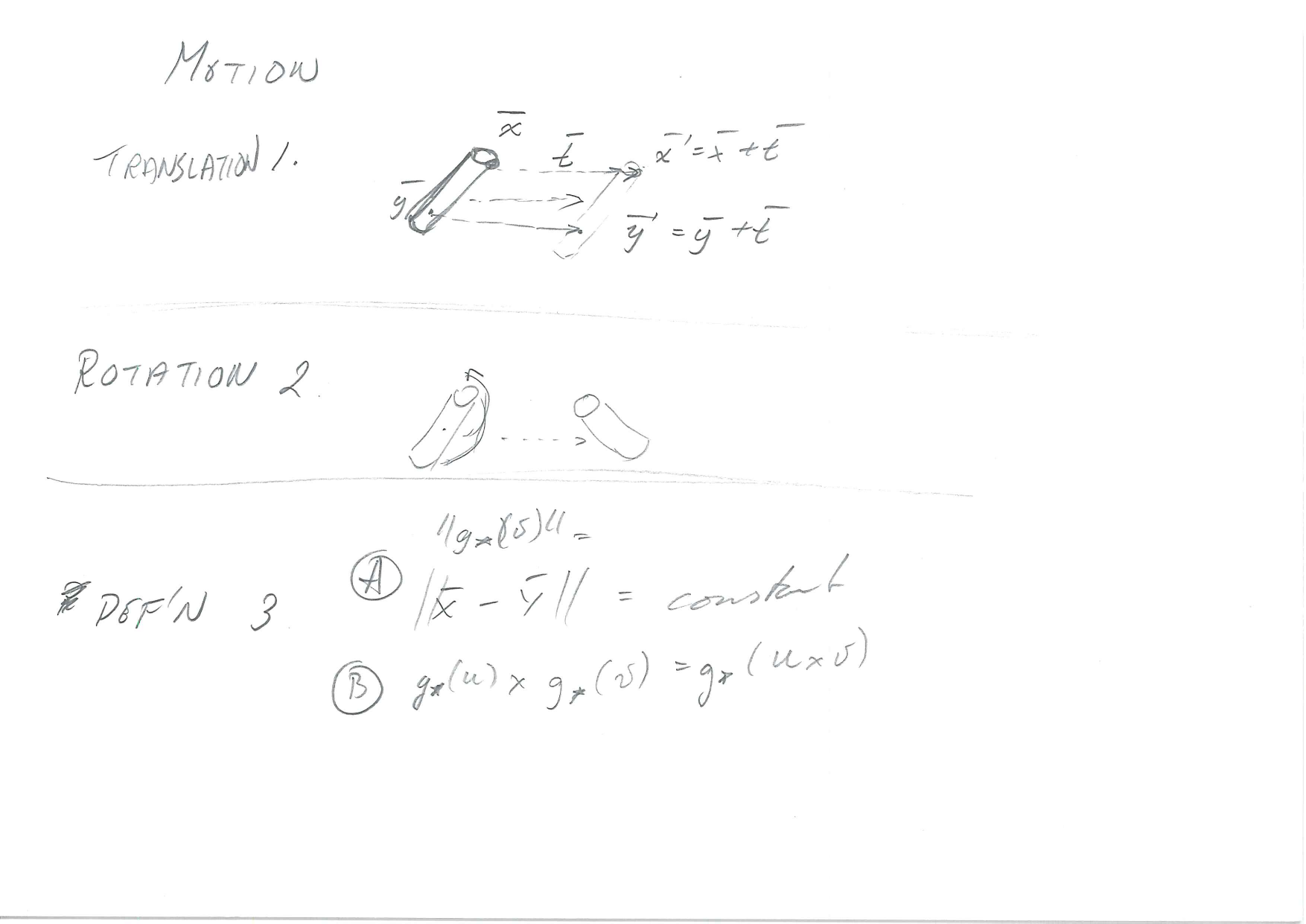
Definition: Rigid Body Motion
- 3D Object is a set of points in \(\mathbb{R}^3\)
- If the object moves, the constituent points move
- The points have to move so that they preserve the shape of the object
Constraints
Let \(\vec{X}(t)\) and \(\vec{Y}(t)\) be the coordinates of points \(\vec{x}\) and \(\vec{x}\) at time \(t\).
- Preserve distance between points
- \(||\vec{X}(t)-\vec{Y}(t)||\) is constant
- cf. magnification example where distance increases.
- Preserve orientation
- c.f. mirroring example
- axes as left hand and right hand systems
- your right hand cannot be rotated to become a left hand
- we have to preserve cross-products
- remember the right hand rule
- If the right hand rule turns into a left hand rule, we have had mirroring.
Let \(u=\vec{X}-\vec{Y}\) be a vector, and \(g_*(u)=g(\vec{X})-g(\vec{Y})\) the corresponding vector after motion.
Preserving the cross-product means \[g_*(u)\times g_*(v) = g_*(u\times v), \forall u,v\in\mathbb{R}^3\]
Change of Basis
Bases
- Basis aka. frame
- Unit vectors: \(\vec{e}_1\), \(\vec{e}_2\), \(\vec{e}_3\)
- The meaning of a tuple to denote a vector
- \(\vec{x}=[x_1,x_2,x_3]= x_1\cdot\vec{e}_1+x_2\cdot\vec{e}_2+x_3\cdot\vec{e}_3\)
- The co-ordinate system is a basis which can be used to define any other vector with a tuple
- The choice of basis is arbitrary
- Any set of three linearly independent vectors \(\vec{u}_1\), \(\vec{u}_2\), \(\vec{u}_3\) can be used as a basis.
- Orthonormal frame: orthogonal and unit length \[\vec{e}_i\vec{e}_j=\delta_{ij} =
\begin{cases}
1 \quad\text{if } i=j\\
0 \quad\text{if } i\neq j
\end{cases}
\]
- Usually, we prefer an orthonormal basis, i.e.
- For orthonormal frames, you can check that all the usual arithmetics work out the same for tuples \(\vec{x}=[x_1,x_2,x_3]\) and for vector sums \(x_1\cdot\vec{e}_1+x_2\cdot\vec{e}_2+x_3\cdot\vec{e}_3\)
- The basis is relative to a given Origin
- i.e. the vectors are not free vectors
Many notatios for the inner product \[\vec{x}\cdot\vec{y} = \vec{x}\vec{y} = \langle\vec{x}, \vec{y}_j\rangle\]
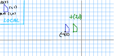
Local and Global Basis
- 3D Scenes are built hierarchically
- Each object is described in a local basis
- and then placed in the global basis.
- Why?
- Save computational work
- Local changes affect only local co-ordinates
- Component motion independent of system motion
Describing a Scene
- Each object described in its own basis
- independently of its position and orientation in the scene
- reusable objects
- Rotation and Deformation can be described locally
- Transformation from local to global co-ordinates
- Rotation of the basis
- Translation of the origin
- System of Systems
- an object in the scene may itself be composed of multiple objects with different local frames
Example
E.g. our co-ordinates: 62°28’19.3“N 6°14’02.6”E
Are these local or global co-ordinates?
Working with Different Bases
Consider common origin first.
Rotating the Basis
- Point \(\vec x\) represented in a basis \(\vec{e}_1\), \(\vec{e}_2\), \(\vec{e}_3\)
- i.e. \(\vec x = x_1\vec{e}_1 + x_2\vec{e}_2 + x_3\vec{e}_3\)
- Translate to a representation in another basis \(\vec{u}_1\), \(\vec{u}_2\), \(\vec{u}_3\)
- Suppose we can write the old basis in terms of the new one
- \(\vec{e_i} = e_{i,1}\vec{u}_1 + e_{i,2}\vec{u}_2 + e_{i,3}\vec{u}_3\)
\[\begin{split} p = & x_1(e_{1,1}\vec{u}_1 + e_{1,2}\vec{u}_2 + e_{1,3}\vec{u}_3) + \\ & x_2(e_{2,1}\vec{u}_1 + e_{2,2}\vec{u}_2 + e_{2,3}\vec{u}_3) + \\ & x_3(e_{3,1}\vec{u}_1 + e_{3,2}\vec{u}_2 + e_{3,3}\vec{u}_3) \\ = &(x_1e_{1,1} + x_2e_{2,1} + x_3e_{2,1} )\vec{u}_1 + \\ &(x_1e_{1,2} + x_2e_{2,2} + x_3e_{2,2} )\vec{u}_2 + \\ &(x_1e_{1,3} + x_2e_{2,3} + x_3e_{2,3} )\vec{u}_3 \end{split}\]
Write \([x'_1, x'_2, x'_3]^\mathrm{T}\) for the coordinates in terms of the new basis.
\[ x'_i = x_1e_{1,i} + x_2e_{2,i} + x_3e_{2,i} \]
- In matrix form we can write \[p = [x_1',x_2',x_3'] = [ \vec{e}_1 | \vec{e}_2 | \vec{e}_3 ]\cdot\vec{x}\] where \(\vec{e}_i\) are written as column vectors.
Note working with a single basis, we can equate a geometric point \(p\) with its vector representation \([x_1,x_2,x_3]\) in the basis. Working with several bases, we need to be careful. One point \(p\) has many representations \(\vec{x}\), one in each basis.
We need to remember that we are describing points in space, and the points do not change just because we describe them differently.
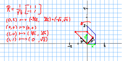
Orthonormal matrix
\[R = [ \vec{e}_1 | \vec{e}_2 | \vec{e}_3 ]\]
- Orthonormal basis means that \(R\cdot R^T = R^T\cdot R=I\)
- Hence \(R^{-1}=R^T\)
- If \(\vec{x}'=\vec{x}\cdot R\) then \(\vec{x}=\vec{x}'\cdot R^T\) then
- If the columns of \(R\) make up the new basis,
- then the rows make up the old basis
Example
\[ \begin{split} R = \begin{bmatrix} \frac{\sqrt{2}}{2} & -\frac{\sqrt{2}}{2} & 0 \\ \frac{\sqrt{2}}{2} & \frac{\sqrt{2}}{2} & 0 \\ 0 & 0 & 1 \end{bmatrix} \end{split} \]
Note this is orthogonal. Compare it to
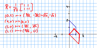
Example in 2D
The principle is the same in 2D.
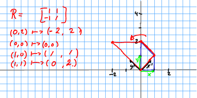
\[ R_1 = \begin{bmatrix} \frac{\sqrt{2}}{2} & -\frac{\sqrt{2}}{2} \\ \frac{\sqrt{2}}{2} & \frac{\sqrt{2}}{2} \\ \end{bmatrix} \quad R_2 = \begin{bmatrix} \frac{\sqrt{2}}{2} & \frac{\sqrt{2}}{2} \\ \frac{\sqrt{2}}{2} & -\frac{\sqrt{2}}{2} \\ \end{bmatrix} \]
Note that
- \(\frac{\sqrt2}{2}=\sin(\pi/4)=\cos(\pi/4)\).
- \(R_1^TR_1=I\) and \(R_2R_2=I\)
- The determinants \(|R_1|=1\) and \(|R_2|=-1\)
Consider a triangle formed by the points \((0,0)\), \((0,1)\), \((1,1)\), and consider each of them rotated by \(R_1\) and \(R_2\)
Rotation around an axis
A rotation by an angle \(\theta\) around the origin is given by \[ R_\theta = \begin{bmatrix} \cos\theta & -\sin\theta \\ \sin\theta & \cos\theta \\ \end{bmatrix} \] In 3D, we can rotate around a given axis, by adding a column and row to the 2D matrix above. E.g. to rotate around the \(y\)-axis, we use \[ R_\theta = \begin{bmatrix} \cos\theta & 0 & -\sin\theta \\ 0 & 1 & 0 \\ \sin\theta & 0 & \cos\theta \\ \end{bmatrix} \]
Operations on rotations
- If \(R_1\) and \(R_2\) are rotational matrices, then \(R=R_1\cdot R_2\) is a rotational matrix
- There is an identity rotation \(I\)
- If \(R_1\) is a rotational matrices, then there is an inverse rotation \(R_1^{-1}\)
- If \(R_1\), \(R_2\), and \(R_3\) are rotational matrices, then \(R_1(R_2R_3)= (R_1R_2)R_3\)
- The set of all rotation matrices in 3D form a group known as \(SO(3)\).
Rotation as Motion
Why is change of basis so important?
- It also describes rotation of rigid bodies
- To rotate a body, rotate its local basis
- Any orthonormal basis is a rotation of any other
- The matrix \(R\) defines the rotation
- Any orthogonal matrix defines a rotation
Demo
Moving the Origin
- A point is described relative to the origin
\[\mathbf x = \mathbf{0} + x_1\cdot\vec{e}_1 + x_2\cdot\vec{e}_2 + x_3\cdot\vec{e}_3\]
- Note that I write \(\mathbf{x}\) for a point and \(\vec{x}\) for a vector
- The origin is arbitrary
- The local co-ordinate system is defined by
- the basis \(\vec{e}_1\), \(\vec{e}_2\), \(\vec{e}_3\)
- the origin \(\mathbf{0}\)
- Move origin: \(\mathbf{0}'=\mathbf{0}+\vec{t}\)
- for some translation vector \(\vec{t}\)
Arbitrary motion
- \(\mathbf{X}\mapsto \mathbf{X}\cdot R + \vec{t}\)
- or \(\mathbf{X}\mapsto (\mathbf{X}-\vec{t}_1)\cdot R + \vec{t}_2\)
- remember, what is the centre of rotation?