Briefing Filters

Reading Szeliski Chapter 3.2

The exercises today are about exploration. If the exercises seem trivial, you should feel free to look beyond. However, make sure that you get used to the processes of finding and using test images from different sources, making filters (as matrices) manually, and applying them in python. These are skills you will need for the next session.

Exercise 1. A simple blurring filter.

In addition to OpenCV, we need numpy for arrays and the signal processing library from SciPy.

import cv2 as cv
import numpy as np
import scipy.signal as sig

(If you have not already installed scipy, you need to do so, e.g. with pip install scipy.)

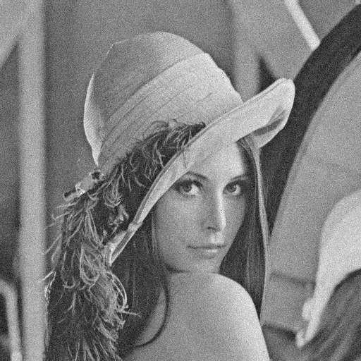
We need a test image which we convert to greyscale. Here we use lenna.ppm, which you have to download and place in your working directory.

frame =cv.imread( "lenna.ppm" )
grey = cv.cvtColor(frame, cv.COLOR_BGR2GRAY)

Other test images can be found at the same source.

We display the image to check that everything works:

cv.imshow("img",grey)
cv.waitKey(0)

Averaging pixels

1. Consider the following python code. What does it do?

(n,m) = grey.shape
new = np.zeros((n-6,m-6),dtype=np.uint8)

for i in range(n-6):
   for j in range(m-6):
      orig = grey[i:i+7,j:j+7]
      new[i,j] = round(sum(orig.flatten())/49)

2. Run the python code. What does the matrix new look like?
3. Display new as an image and compare it to the original grey. What is the visual effect?

What you should observe is a blurring effect.
Contours are smoothened by averaging a neighbourhood.

Exercise 2. Using a signal processing library

What we did above is such a standard operation that we have an API therefore. We can define a \(7\times7\) averaging filter like this.

f7 = np.ones((7,7)) /  49

• What does this look like as a matrix?

To apply the filter to the image, we can use the standard convolution operator as follows:

g7 = sig.convolve2d(grey,f7).astype(np.uint8)

Note that we have to convert the result to integers explicitly, lest OpenCV will not interpret it as an image. The result can be displayed as

cv.imshow("filtered",g7)
cv.waitKey(0)

• Compare the two images. What does the filter do?
• Compare the filtered image to the image new from your manual averaging. Do they look different in any way?

The API has different methods to handle the boundaries.
We simply cropped a few pixel around the border, and thus new may be smaller than images filtered with the API.

We can do the same thing using the OpenCV library, like this.

c7 = cv.filter2D(grey,-1,f7)

The second argument (-1) specifies the colour depth of the output which should be the same as for the input.

Other tests

1. Download Images/lenna-awgn.png and Images/lenna-snp.png. These are noisy versions. What do the images look like?
2. Test the above filter on the noisy images. What do you get?
3. Try different averaging filters instead of f7. Try for instance \(3\times3\) and \(5\times5\) filters. (Remember to change the normalisation factor (49) so that you get a zero-sum matrix.) Do you get good denoising results?

Disc filter

Sometimes a disc-like filter is used, like this.

circle = np.array([[0,0,1,1,1,0,0],
   [0,1,1,1,1,1,0],
   [1,1,1,1,1,1,1],
   [1,1,1,1,1,1,1],
   [1,1,1,1,1,1,1],
   [0,1,1,1,1,1,0],
   [0,0,1,1,1,0,0]])/37

Test it. Which filters give the best denoising effects?

Exercise 3. A Gaussian filter

The Gaussian filter is a little trickier to implement, since we want to be able to vary its parameters. We use the Gaussian function \[g(x,y) = \frac{1}{2\pi\sigma^2}\exp\frac{-(x^2+y^2)}{2\sigma^2},\] where \(\sigma\) is the standard deviation and \((x,y)\) is the pixel co-ordinates with \((0,0)\) in the centre of the filter.

Firstly, the Gaussian function in python becomes

def gauss(x,y,sigma=1):
    c1 = 1/(2*np.pi*sigma**2)
    c2 = 2*sigma**2
    return c1*np.exp(-(x**2+y**2)/c2)

1. Check that the above code matches the mathematical formula.

We can make a list of lists of Gaussian coefficients in a simple one-liner:

B = [ [ gauss(x,y) for x in range(-t,t+1) ] for y in range(-t,t+1) ]

where t is an integer and the resulting filter is \((2t+1)\times(2t+1)\).

2. How does the above code work?
3. It may be useful to plot the Gaussian as a surface plot in matplotlib.
   • If you do not know how, you can use the method from the video on image representation, where we plotted the image as a surface plot of a function. The object B or the matrix A below can be plotted in the same way.

To turn B into a matrix, we do

A = np.array(B)

3. Make the matrix A. What does the matrix look like?

4. The elements of the filter should add to one, to maintain the luminence of the image. You can check this by calculating A.sum(). What do you think, is this sufficiently close to one? Why is it less than one?

5. We can normalise the filter by calculating AA = A/A.sum(). Why does this give a matrix with unit sum?

6. Now, test the Gaussian filter on your test images. Use a couple of different sizes, e.g. \(t=3,7,11\), and a couple of different standard deviations, e.g. \(\sigma=0.5,1,2\). What do you observe?

Remark

Sometimes the following approximation is used for a Gaussian filter. Feel free to test it if you have time.

\[\frac{1}{16} \begin{bmatrix} 1 & 2 & 1 \\ 2 & 4 & 2 \\ 1 & 2 & 1 \\ \end{bmatrix} \]

Exercise 4. Noisy images

You can try to make your own noisy images using the code below.

1. How does each code snippet work?
2. Apply the functions to different images to make noise versions.
3. Test your blur filters on different images. Is there a blur filter which always works best?

Gaussian Noise

(m,n) = grey.shape
noise = np.random.randn(m,n)*sigma
noisy = (grey + noise).astype(np.uint8)

def gnoise(img,sigma=1):
     (m,n) = grey.shape
     noise = np.random.randn(m,n)*sigma
     return (grey + noise).astype(np.uint8)

Salt noise

def snoise(img,p=0.1):
     (m,n) = grey.shape
     noise = (np.random.rand(m,n) > (1-p)).astype(np.uint8)*255
     return np.maximum(grey,noise)

Pepper noise

def pnoise(img,p=0.1):
     (m,n) = grey.shape
     noise = (np.random.rand(m,n) > p).astype(np.uint8)*255
     return np.minimum(grey,noise)

Exercise 5. A teaser for next section (optional)

Consider the following filters.

\[\begin{bmatrix} 0 & 1 & 0 \\ 1 & -4 & 1 \\ 0 & 1 & 0 \end{bmatrix} \quad \begin{bmatrix} 1 & 0 & -1 \\ 2 & 0 & -2 \\ 1 & 0 & -1 \end{bmatrix} \quad \begin{bmatrix} 1 & 2 & 1 \\ 0 & 0 & 0 \\ -1 & -2 & -1 \end{bmatrix} \]

1. Test these filters. What is the result?

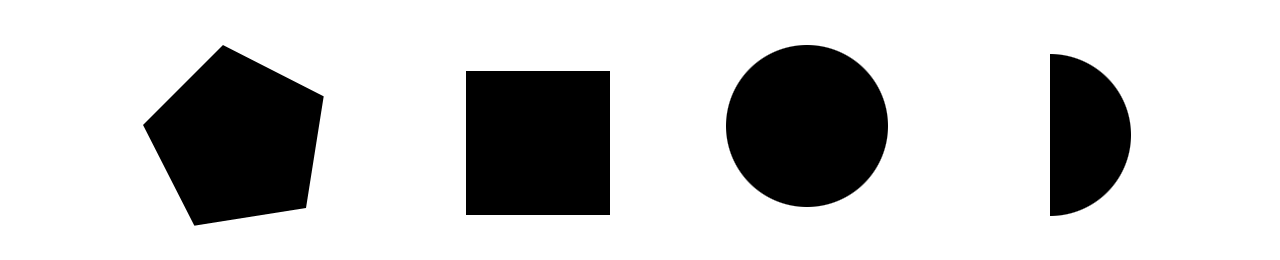
It will be useful to test on simple geometrical shapes, like the image in this post (in addition to ordinary fotographs). Note, however, that the transparent background can cause problems. This image has had the background changed to white, using ImageMagick as follows:

convert Images/shapes.png -background white -alpha remove -alpha off shapes.png

2. Test the filters on the shapes image.

Note that these filters do not preserve the range of pixel values. If the depth is originally \([0,1]\), these filters give a range of \(\pm4\). We can try to deal with this as follows.

3. Normalise the filters by dividing by 8. What range would the images get now?
4. Add \(0.5\) to the the resulting image matrix, which gives what range?
5. What do the filtered images look like now?

These filters work as edge detectors. More about this next session.

Exercise 6. Further exploration (optional)

1. Take an image with your built-in camera and test your denoising filters thereon.
2. Look up openCV and other python libraries. What built-in blur filters can you find?
   Are there any ready-made APIs to simplify the above exercises?
3. You may want to inspect my Sample Code. It does approximately what we have done above, but the code is cleaned up for use on the command line.

Reflection

1. Review today’s tutorial. What are the key concepts that you want to take with you?
2. Next week we will introduce a new set of filters for differentiation of the image.
   Each filter is defined by a relatively small matrix. What do you need to change in the above examples to use different filters?
3. What does the filter size matter? For instance, how does the blurred image change when you decrease the size of the averaging filter from \(7\times\) to \(3\times3\)?