Reading

• Ma 2004 Chapter 1.

Session

1. Briefing Overview and History
2. Install and Test Software
   • Simple tutorials
3. Debrief questions and answers
   • recap of linear algebra

1 Briefing

Practical Information

Information

• Wiki - living document - course content
• BlackBoard - announcements - discussion fora
• Questions - either
  • in class
  • in discussion fora
• Email will only be answered when there are good reasons not to use public fora.

Taught Format

• Sessions 4h twice a week
  • normally 1h briefing + 2h exercise + 1h debrief (may vary)
• Exercises vary from session to session
  • mathematical exercises
  • experimental exercises
  • implementational exercises
• No Compulsory Exercises
• Feedback in class
  • please ask for feedback on partial work
• Keep a diary. Make sure you can refer back to previous partial solution and reuse them.

Learning Outcomes

• Knowledge
  • The candidate can explain fundamental mathematical models for digital imaging, 3D models, and machine vision
  • The candidate are aware of the principles of digital cameras and image capture
• Skills
  • The candidate can implemented selected techniques for object recognition and tracking
  • The candidate can calibrate cameras for use in machine vision systems
• General competence
  • The candidate has a good analytic understadning of machine vision and of the collaboration between machine vision and other systems in robotics
  • The candidate can exploit the connection between theory and application for presenting and discussing engineering problems and solutions

Exam

• Oral exam \(\sim 20\) min.
• First seven minutes are yours
  • make a case for your grade wrt. learning outcomes
  • your own implementations may be part of the case
  • essentially that you can explain the implementation analytically
• The remaing 13-14 minutes is for the examiner to explore further
• More detailed assessment criteria will be published later

Vision

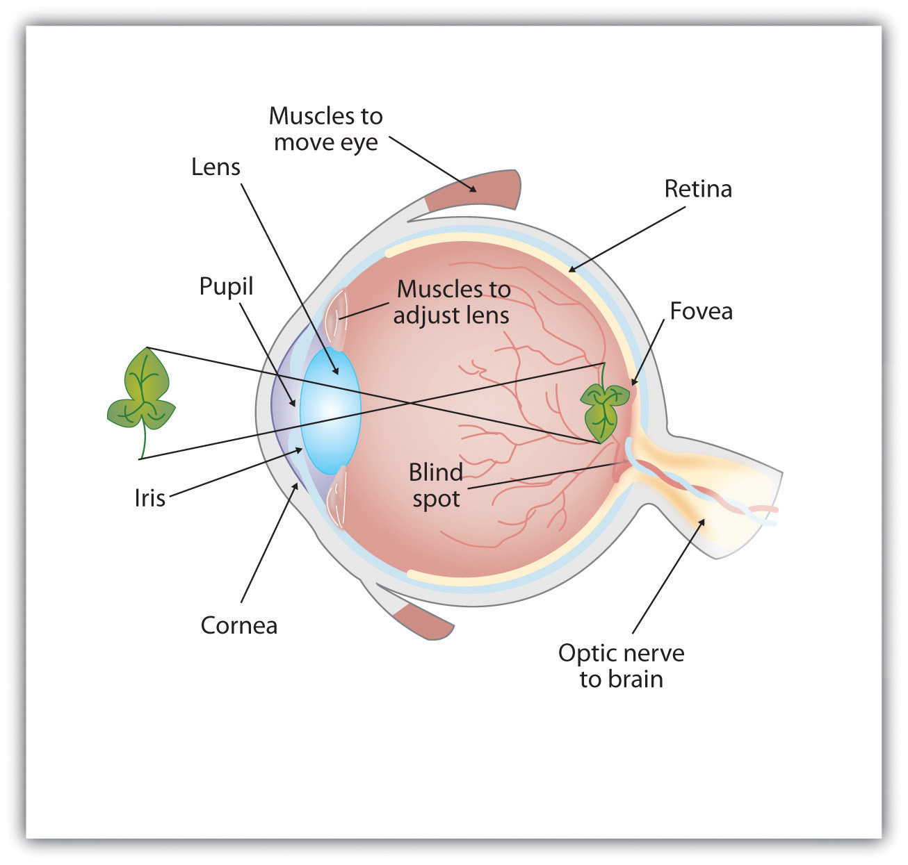
• Vision is a 2D image on the retina
  • Each cell perceives the light intencity of colour of the light projected thereon
• Easily replicated by a digital camera
  • Each pixel is light intencity sampled at a given point on the image plane

Cognition

Cognition

• 3D model - cognitive schemata
• 2D image on the retina
• why is the correspondence difficult?
• history of machine vision

2 Lab Practice

The most important task today is to install and test a number of software packages needed.

Install Python

We will use Python 3 in this module. You need to install the following.

1. Python
2. pip. (the package manager for python)
3. iPython (a more convenient interactive interpreter)

How you install these three packages depends on your OS. In most distroes you can use the package system to install all of this, for instance in Debian/Ubuntu:

sudo apt-get install ipython3 python3-pip

(Python is installed automatically as a dependency of iPython3. Note, you have to specify version 3 in the package names, lest you get Python 2.)

Install Python Packages

Python packages are installed most easily using python’s own packaging tool, pip, which is independent of the OS. It is run from the command line.

Depending on how you installed pip, it may be a good idea to upgrade

pip3 install --upgrade pip

Then we install the libraries we need. You can choose to install either in user space or as root.

User space:

pip3 install --user matplotlib numpy opencv-python

As root:

sudo pip3 install matplotlib numpy opencv-python

• numpy is a standard library for numeric computations. In particular it provides a data model for matrices with the appropriate arithmetic functions.
• matplotlib is a comprehensive library for plotting, both in 2D and 3D.
• OpenCV is a Computer Vision library, written in C++ with bindings for several different languages.

A third installation alternative is to use Virtual Environments, which allows you to manage python versions and dependencies separately for each project. This may be a good idea if you have many python projects, but if this is your first one, it is not worth the hassle.

Run iPython

Exactly how you run iPython may depend on you OS. In Unix-like systems we can run it straight from the command line:

ipython3

This should look something like this:

georg$ ipython3 
Python 3.7.3 (default, Jul 25 2020, 13:03:44) 
Type 'copyright', 'credits' or 'license' for more information
IPython 7.3.0 -- An enhanced Interactive Python. Type '?' for help.

In [1]: print("Hello World")                                                    
Hello World

In [2]: import numpy as np                                                      

In [3]: np.sin(np.pi)                                                           
Out[3]: 1.2246467991473532e-16

In [4]: np.sqrt(2)                                                              
Out[4]: 1.4142135623730951

In [5]:                                                                         

Some 3D Operations

In this chapter, we will define a simple 3D Object and display it in python. The 3D object is an irregular tetrahedron, which has four corners and four faces.

import numpy as np
from matplotlib import pyplot as plt
from mpl_toolkits.mplot3d.art3d import Poly3DCollection

Firtsly, we define the three corners of the tetrahedron.

corners = [ [-1,0.5,0.5], [+1,0.5,0.5], [0,-0.5,0.5], [0,0.5,-0.5] ]

Each face is adjacent to three out of the four corners, and can also be defined by these corners.

face1 = [ corners[0], corners[1], corners[2] ] 
face2 = [ corners[0], corners[1], corners[3] ] 
face3 = [ corners[0], corners[2], corners[3] ] 
face4 = [ corners[1], corners[2], corners[3] ] 

To represent the 3D structure for use in 3D libraries, we juxtapose all the faces and cast it as a matrix.

vertices = return np.array(face1+face2+face3+face4,dtype=float)
print(vertices)

Observe that the vertices (corners) are rows of the matrix. The mathematical textbook model has the corners as columns, and this is something we will have to deal with later.

We define the 3D object ob as follows.

ob = Poly3DCollection(vertices, linewidths=1, alpha=0.2)

The alpha parameter makes the object opaque. You may also want to play with colours:

ob.set_facecolor( [0.5, 0.5, 1] )
ob.set_edgecolor([0,0,0])

To display the object, we need to create a figure with axes.

plt.ion()
fig = plt.figure()
ax = fig.add_subplot(111, projection='3d')
plt.show()

Note the plt.ion() line. You do not use this in scripts, but in ipython it means that control returns to the prompt once the figure is shown. It is necessary to continue modifying the plot after it has been created.

Now, we can add our object to the plot.

ax.add_collection3d(ob)

Quite likely, the object shows outside the range of the axes. We can fix this as follows:

s = [-2,-2,-2,2,2,2]
ax.auto_scale_xyz(s,s,s)

These commands make sure that the axes are scalled so that the two points (-2,-2,-2) and (2,2,2) (defined in the list s) are shown within the domain.

Rotation and Translation of 3D objects

TODO

Some Camera Operations

import numpy as np
import cv2 as cv
cap = cv.VideoCapture(0)
ret, frame = cap.read()

Now, ret should be True, indicating that a frame has successfully been read. If it is False, the following will not work.

gray = cv.cvtColor(frame, cv.COLOR_BGR2GRAY)
cv.imshow('frame', gray)
cv.waitKey(1) 

You should see a greyscale image from your camera. To close the camera and the window, we run the following.

cap.release()
cv.destroyAllWindows()

3 Debrief