Exercises

Equivalence of Points (Based on Exercise 3.1.)

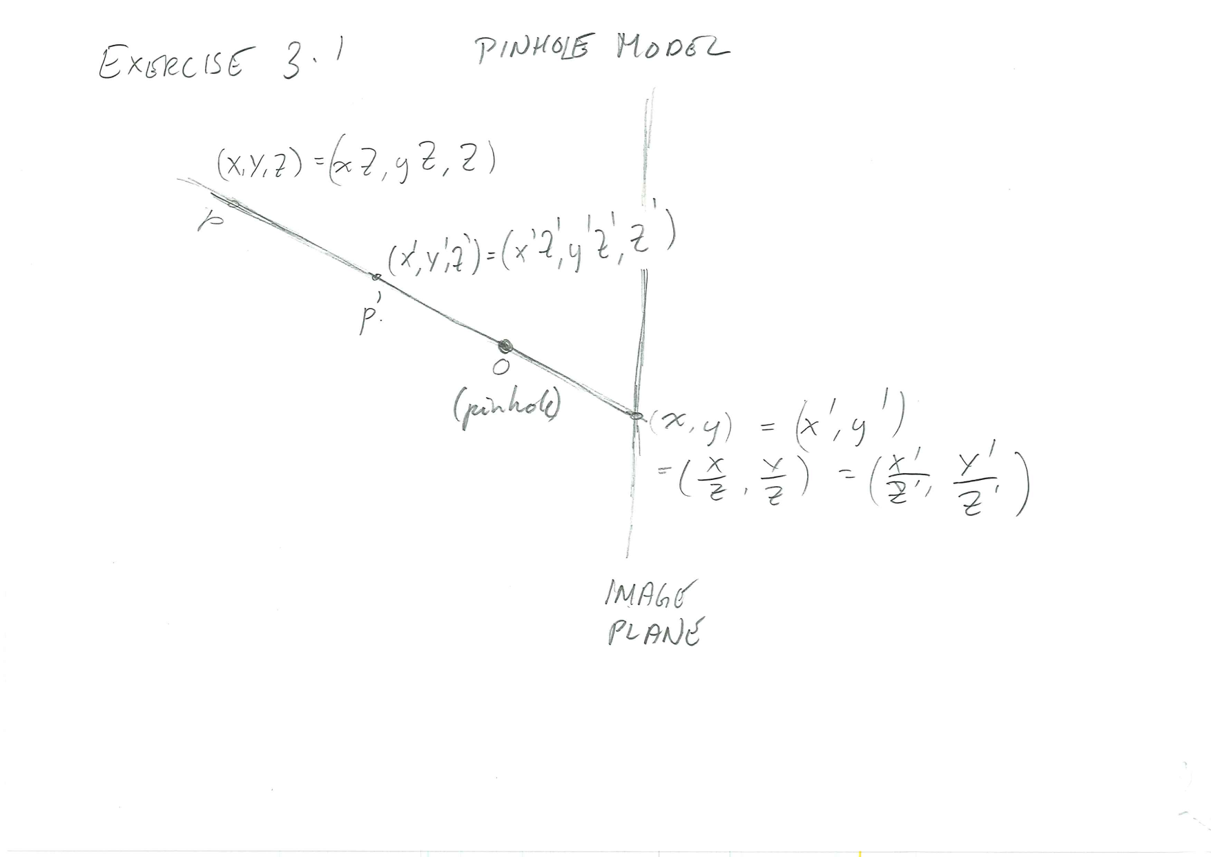
Note that the thin lens model is similar since rays through the centre of the lens (optical centre) are not deflected, and thus serves the role of a pinhole.

(Exercise 3.2)

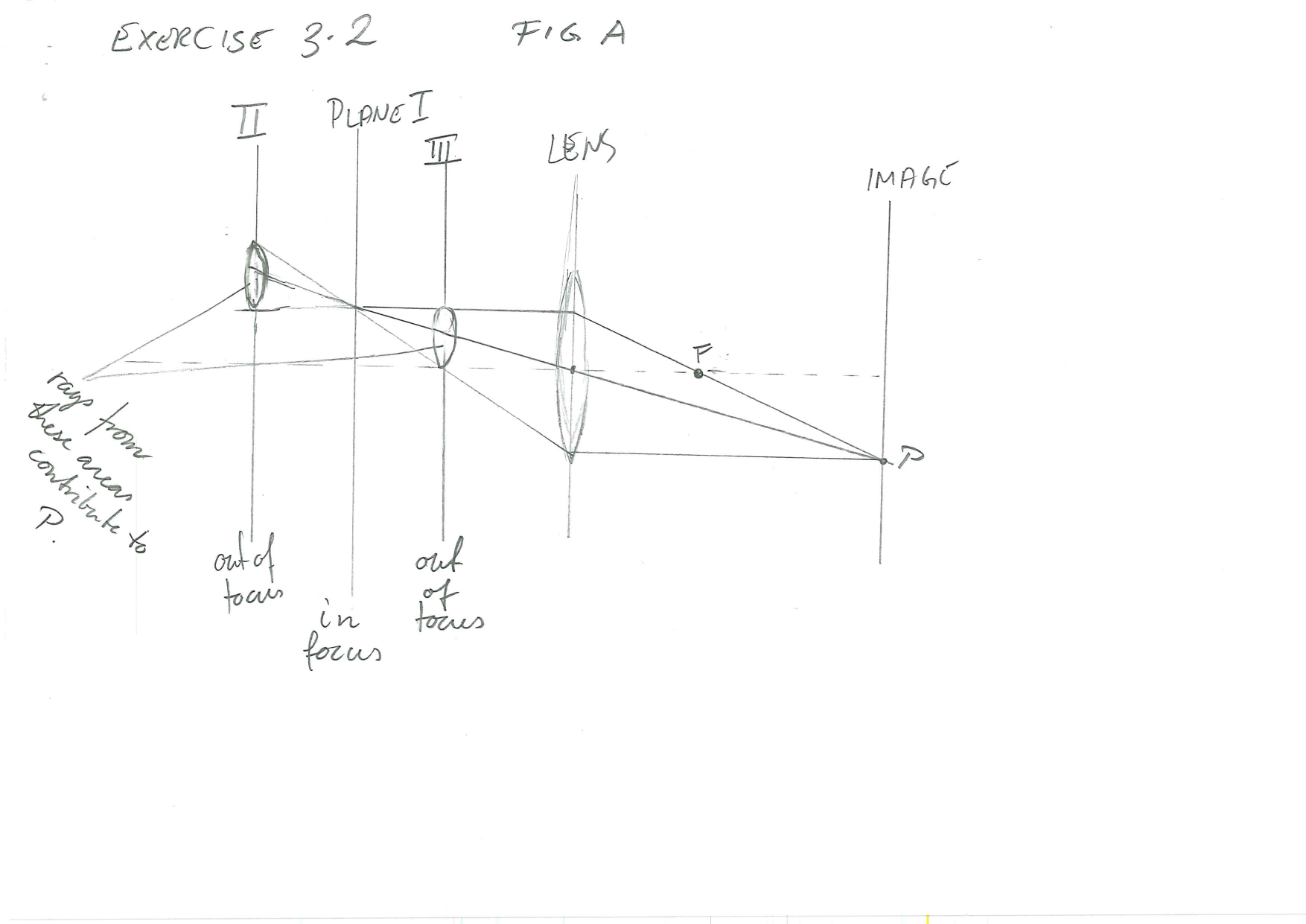
This initial figure is slightly inaccurate. Horizontal lines (object to lens, and lens to image point) delimit the region of interest. In reality it is the aperture that delimits the bundle of light that contributes to the image.

However it was my first impression of a possible solution, and if we just image that the aperture just happens to extend exactly to cover the rays drawn, then it is fine. Let’s redraw.

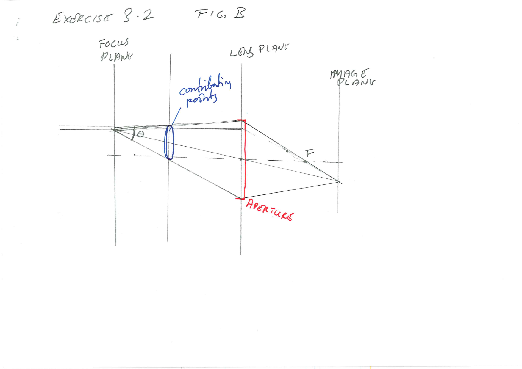
The second model shows the bundle of light emanating from the object point in the focus plane and passing through the apperture. Assuming that the aperture is is circular, the bundle is a skew cone, and the points contributing to the image point from the out-of-focus plane is a section of the skew cone.

This may sound as if we have to dig deep into Geometry and not only read the theory of conic sections but also the extensions to skew cones. Luckily, it is a lot simpler. Let’s redraw the figure, naming the points for ease of discussion.

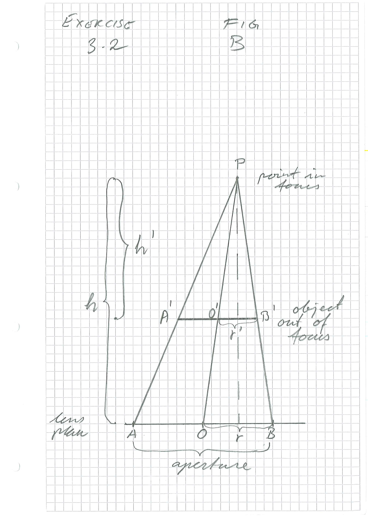
The drawing of the skew cone shows cross-section through the top \(P\) and the centre \(O\) of the base, but the argument can be made with any such cross-section. The line segments \(AO\) and \(BO\) are equal to the radius of the aperture in every cross-section, and the aperture is a circle, so the radius is always the same. Thus, even if the angle at \(P\) is different, the lengths \(AO\) and \(BO\) are constant.

We know that \(A'B'\) is parallell to \(AB\). Hence the triangles \(A'B'P\) and \(ABP\) are equivalent. The same is the case for \(A'O'P\) versus \(AOP\) and \(B'O'P\) versus \(BOP\). It follows that the ratio of the heights is equal to the ratio of the bases, that is: \[\frac{h'}{h} = \frac{A'O'}{AO} = \frac{B'O'}{BO}\] Since \(AO=BO=r\) is the radius of the aperture, \(A'O'=B'O'\) is the radius of the object. Hence the object forms a circle with radius \(r'=A'O'=B'O'\).
This gives \[\frac{h'}{h} = \frac{r'}{r}\] or \[r'=\frac{h'}{h}\cdot r\] Hence the object that contributes to the image of \(P\) is a circle with radius \(r'=h'r/h\), where \(h'\) is the distance between the focus plane and the object plane.

Bonus Question In the drawings the object is between the plane in focus and the lens. Would we still get \(r'=h'r/h\) if the object is too far away to be in focus?

(You can find the centre of the object using a similar argument. In fact, that would similar to the argument you used in the previous exercise. The new insight is in the part that we have solved.)

I agree that this exercise is tricky, in the sense that the solution is not at all obvious at the start. If you expect to find a template solution you are stuck. I had to make each of the figures in turn without knowing where I would be heading next, just to earn a little more insight into the problem each time. To succeed, you have to focus on understanding the geometry, rather than finding a computational procedure.

Scale Ambiguity (Exercise 3.8).

Use the figure from Exercise 3.1. Ask if it does not suffice.

Field of View (Exercise 3.3 Part 1)

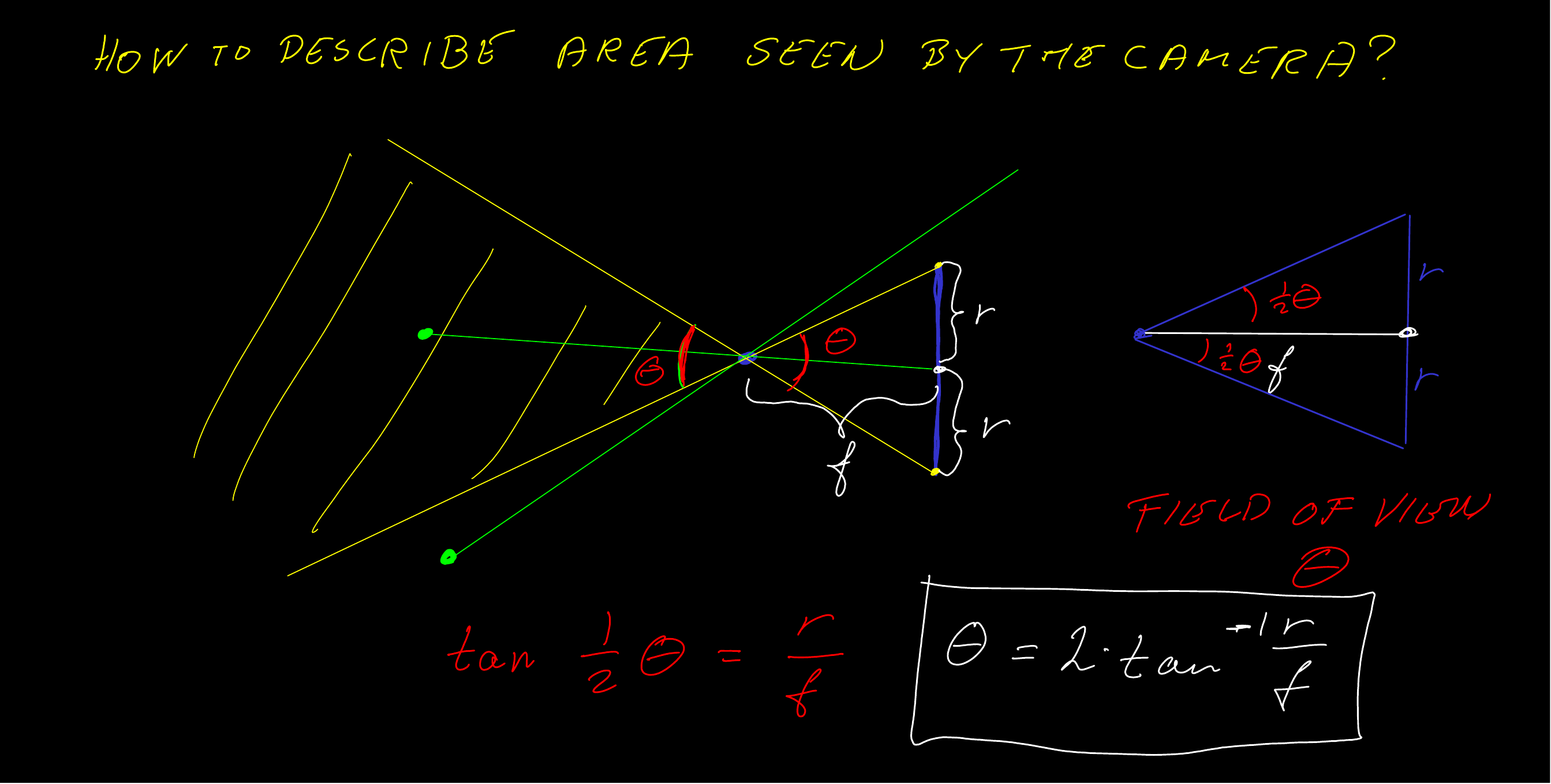
\[\theta = 2\tan^{-1}\frac{r}{f}\]

Exercise 3.3 Part 1-2.

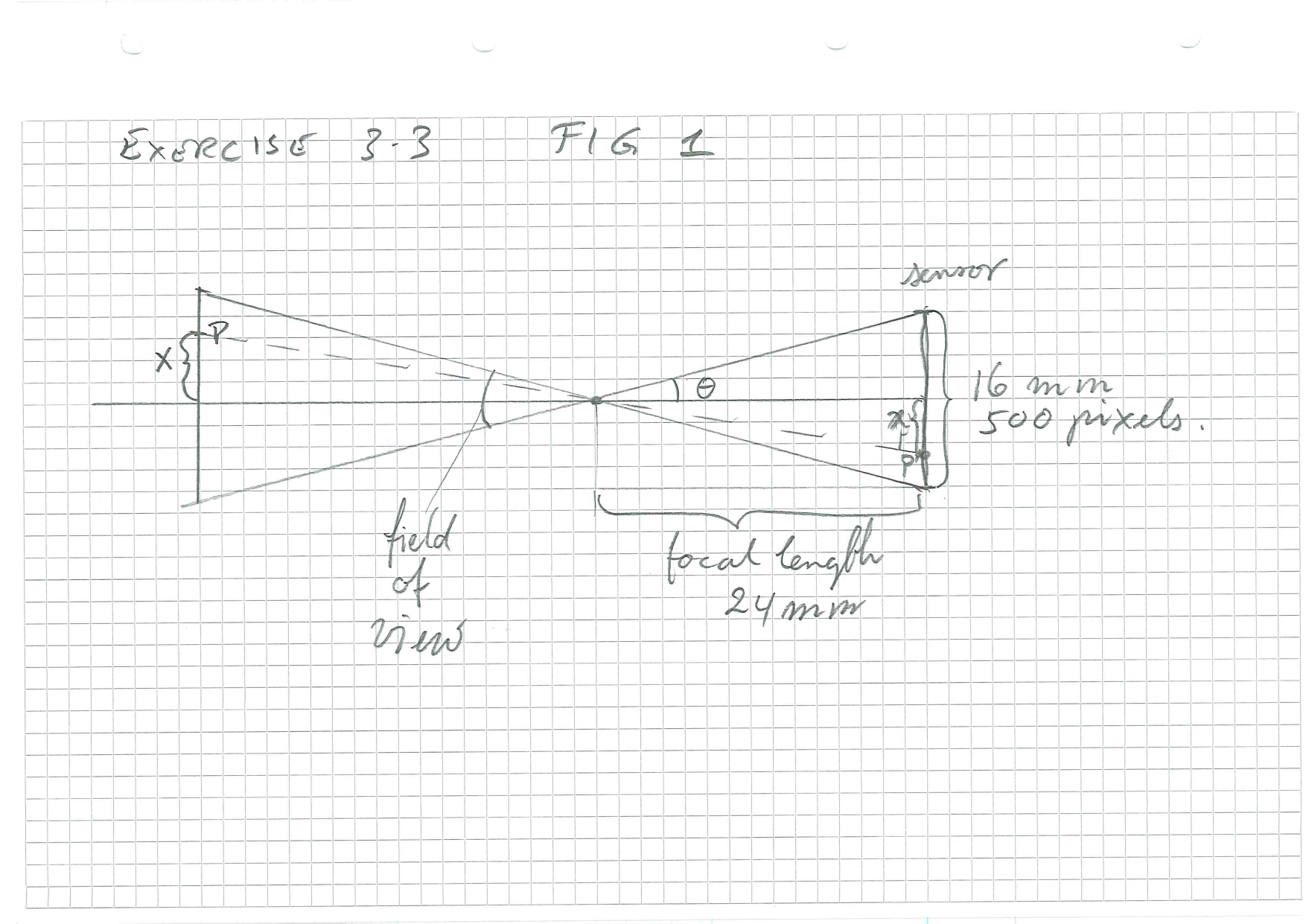
The figure shows a horizontal plane, where you can compute the \(x\) co-ordinates. The field of view is conventionally calculated in the longest dimension which is assumed to be along the \(x\)-axis.

The field of view is \(2\theta\), and \(\theta\) is an angle in a right-angled triangle where you know two sides. Calculation is now basic trigonometry.

To calculate the relationship beween \(x\) (image co-ordinate) and \(X\) (3D object co-ordinate), we have to work in several steps.

1. Firstly, we express the relationship in metric co-ordinates, using the now familiar ideas of congruent triangles.
2. Secondly, we need to translate from metric to pixels.
3. Thirdly, we need to shift the origin, which is normally at the centre in metric terms and the upper left corner in pixel terms.

Since the height and width of the sensor differ, the calculation has to be redone with different numbers for the \(y\)-direction.

Taking it in steps, this should be straight forward.