Revision 5d777b902e99198ab331234a5c9ae936a3a2974f (click the page title to view the current version)
Deep Q-Learning
Slides rl-3.pdf
Briefing
Last week we implemented Q-Learning, which uses a lookup table, defining the Q-Value for every (state,action) pair. This becomes a map \[(\text{state},\text{action}) \mapsto \text{value}\] We can also read it as a map \[\text{state} \mapsto (\text{action},\text{value})\] where the action and value are found by taking the maximum in the row corresponding to the given state.
In Deep Q-Learning we replace the lookup table with a deep neural network. To understand this, we have to see the neural network as a function (or map) \[\text{state} \mapsto (\text{action},\text{value})\] The neural network (or any regression or classification model in general) takes an input and predicts the corresponding output. During training the weights or parameters of the model are tuned to minimise the error on a given training set.
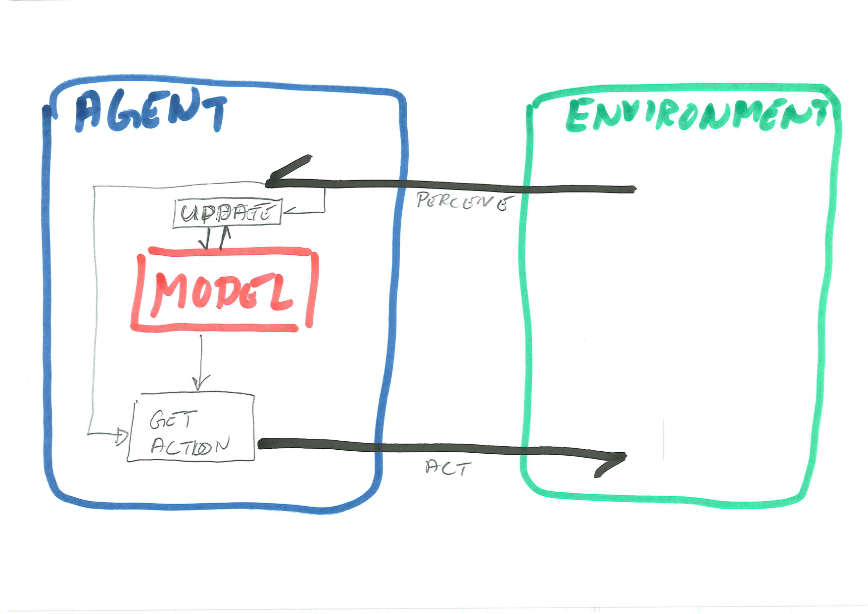
Hence, in the RL Agent in the diagram, the model is a neural network, and the get action operation is simply an evaluation of the network. The tricky part is the update method. Unlike the first textbook demonstrations of machine learning, we cannot pregenerate a training set and train once and for all, because the set of bad solutions is far too large. Instead, we need to use exploration strategies similar hill climbing, so that once we find a half-good state, we explore the neighbourhood for better states.
The tutorial gives only one approach to network update. As is so often the case in machine learning and artificial intelligence, it is far from obvious what will be the best solution in any given case.
It should be noted that Deep Q-Learning is primarily designed for very large, and typically continuous, state spaces. Applying it here on the frozen lake is merely an illustration. It is a useful illustration because we can validate the solution either manuall or by comparison with regular Q-Learning.
Exercise
Task 1 - Tensorflow/Keras
We will start today with getting used to tensorflow/keras, you can also adapt the exercises to pytorch or similar if prefered (but code-examples will be given in tensorflow).
First, install tensorflow:
We will only be using the Keras API, you can find the documentation here
Verify in python with:
Part A - Perceptron
We can make a single perceptron with keras like this:
from tensorflow import keras
from tensorflow.python.keras.layers import Dense

model = tf.keras.Sequential([
  Dense(units=1, input_dim=1)
])
and do a forward propagation with:
Furthermore, we can get and set the current weights with:
# Get weights
model.layers[0].get_weights()

# Set weights (TODO: replace w1 and b1)
model.layers[0].set_weights([np.array([[w1]]), np.array([b1]))
Tasks/Questions - Test out different values for the weight and bias - How do you forward-propogate multiple values at once? - Can you plot the graph for some range of inputs?
Task 2 - Q-Values from an ANN
We still want to work with Q-values, meaning that we would like some value for all possible actions as output from our neural network. Our FrozenLake environment has 4 possible actions, and we already know the q-values for all possible states, making it easy to fit a neural network.
Part A - Creating a network
The following code will create a neural network that inputs a state (one value) and outputs 4 values (one for each action), it will also assume 16 possible states (0-15):
import numpy as np
import tensorflow as tf
from tensorflow import keras
from tensorflow.python.keras.layers import Dense

x_data = np.linspace(0, 15, 16)
normalizer = keras.layers.Normalization(input_shape=[1,], axis=None)
normalizer.adapt(np.array(x_data))

model = keras.Sequential([
	 normalizer,
	 Dense(64, activation='relu'),
	 Dense(64, activation='relu'),
	 Dense(4)
])

model.compile(
    optimizer=tf.optimizers.Adam(learning_rate=0.001),
	  loss='mse'
)
Answer the following:
- What does the
x_datalook like (data type, contents, structure)? This will be used as network input, that is, each element should be a state. - What is the design (structure) of this neural network? Look primarily on the lined defining
model.
The normalizer (which is defined after x_data) scales the input so that all features have the same magnitude.
The model.compile statement defines the optimiser algorithm (tuning the weights) and the loss function (defining the cost of current errors).
Tasks/Questions
Part B - Training
As we already have Q-Values, let us train the network on the data:
y_data = np.array([
	[0.54, 0.53, 0.53, 0.52],
	[0.34, 0.33, 0.32, 0.50],
	[0.44, 0.43, 0.42, 0.47],
	[0.31, 0.31, 0.30, 0.46],
	[0.56, 0.38, 0.37, 0.36],
	[0., 0., 0., 0.],
	[0.36, 0.2, 0.36, 0.16],
	[0., 0., 0., 0.],
	[0.38, 0.41, 0.40, 0.59],
	[0.44, 0.64, 0.45, 0.40],
	[0.62, 0.50, 0.40, 0.33],
	[0., 0., 0., 0.],
	[0., 0., 0., 0.],
	[0.46, 0.53, 0.74, 0.50],
	[0.73, 0.86, 0.82, 0.78],
	[1, 1, 1, 1]
])

model.fit(
	x_data,
	y_data,
	epochs=50000,
	verbose=0)

decisions = model(x_data)
print(decisions)y_datais the Q-table in the format we have used before. Rows correspond to states and columns to actions.model.fittrains the networkmodel(x_data)applies the network to predict the Q-values for each state inx_data.
Discuss/answer the following.
- Test out the forward propagation, are the values similar to what you expect from a Q-table?
- Plot the utility given optimal play. (Do this manually if you do not instantly see how to program it.)
Part C - FrozenLake
Given the model trained above and an optimal policy (argmax of output), can you move around the environment/solve the problem?
Task 3 - DQN
Given exercises from last week, we now only need an implementation of a replay-buffer to implement a DQN (Deep Q-network) agent. The replay-buffer needs two methods, one to store experiences (state, action, reward, next_state), and one to sample from the replay-buffer.
Implement these two methods
Task 4 - MountainCar
Until now we have been working on the FrozenLake environment. Try to solve the MountainCar environment using techniques we have learned in this course.
I will update this page with a DQN-solution later (hopefully before the end of the day).