Vision is the inverse problem of image formation

• perspective

Briefing

The Eye Model

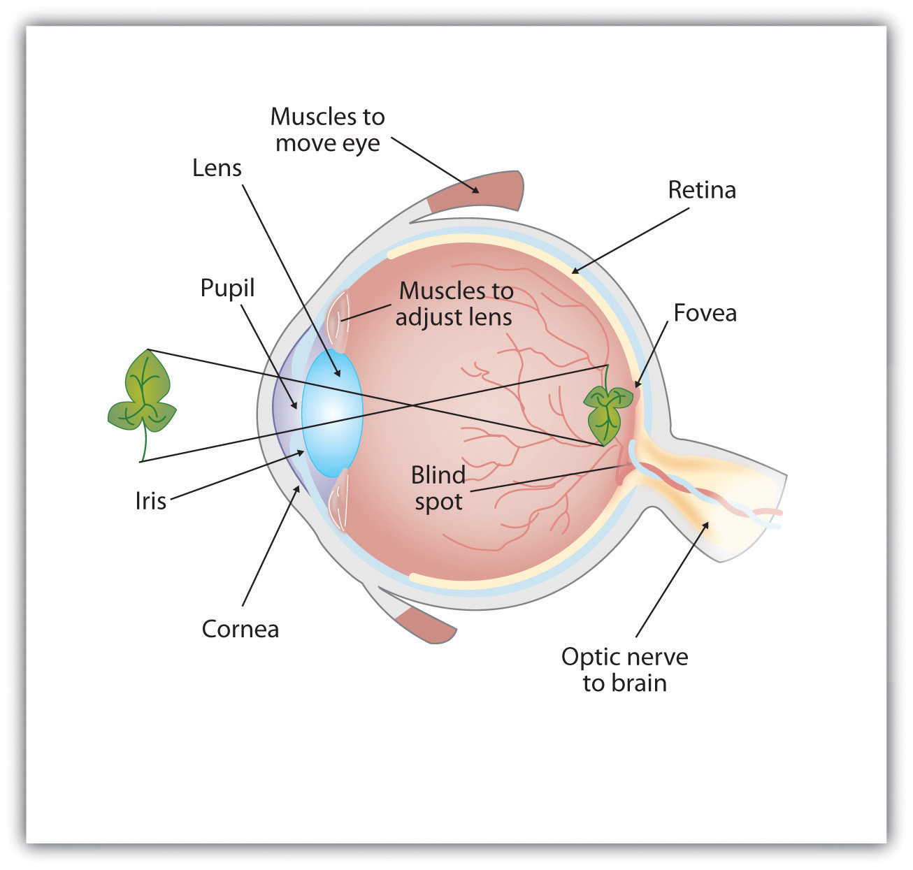
• An image of the real world is projected on the Retina.
• Modern Cameras (more or less) replicate the Eye Model.

Image Representation

The Retina, or image sensor, is able to sense the projected rays.

A fine grid of sensors or perceptive cells is able to measure, or sample, the light intensity falling upon it.

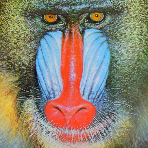
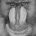
Let’s have a look at the resulting data, using the popular mandrill image shown to the right.

import numpy as np
import cv2 as cv
from matplotlib import pyplot as plt

im = cv.imread("mandrill-grey.png")

Now, we have loaded the image as the object im. Firstly, we observe that this is a matrix.

Out[55]:
array([[[ 76,  76,  76],
        [ 60,  60,  60],
        [ 68,  68,  68],
        ...,
        [ 90,  90,  90],
        [ 97,  97,  97],
        [ 96,  96,  96]],

       [[ 83,  83,  83],
        [ 72,  72,  72],
        [ 77,  77,  77],
        ...,
        [ 99,  99,  99],
        [ 87,  87,  87],
        [106, 106, 106]],

       [[ 51,  51,  51],
        [ 75,  75,  75],
        [117, 117, 117],
        ...,
        [ 99,  99,  99],
        [ 81,  81,  81],
        [ 88,  88,  88]],

       ...,

       [[139, 139, 139],
        [140, 140, 140],
        [136, 136, 136],
        ...,
        [ 92,  92,  92],
        [ 96,  96,  96],
        [ 78,  78,  78]],

       [[131, 131, 131],
        [144, 144, 144],
        [138, 138, 138],
        ...,
        [ 85,  85,  85],
        [ 98,  98,  98],
        [ 90,  90,  90]],

       [[109, 109, 109],
        [102, 102, 102],
        [109, 109, 109],
        ...,
        [ 57,  57,  57],
        [ 67,  67,  67],
        [ 69,  69,  69]]], dtype=uint8)

In [56]: im.shape
Out[56]: (128, 128, 3)

A little confusingly, this matrix has three dimensions, as if it were a colour (RGB) image. Since it is grey scale, we only need one \(128\times128\) matrix. As we see above, the three values in each tripple are equal so we can take one arbitrary plane from the matrix.

Out[58]:
array([[ 76,  60,  68, ...,  90,  97,  96],
       [ 83,  72,  77, ...,  99,  87, 106],
       [ 51,  75, 117, ...,  99,  81,  88],
       ...,
       [139, 140, 136, ...,  92,  96,  78],
       [131, 144, 138, ...,  85,  98,  90],
       [109, 102, 109, ...,  57,  67,  69]], dtype=uint8)

In [59]:

This is the first representation of a grey scale image, as an \(n\times m\) matrix.

OpenCV provides the functions to show the image as an image. This is the second representation of the image.

In [60]: cv.imshow("mandrill grey", im)

In [61]: cv.waitKey(1)
Out[61]: -1

The matrix can also be read as a signal, sampling values \(I(x,y)\) for different values of \(x\) and \(y\). This gives the third representation, as a 3D surface plot.

In [7]: plt.ion()
Out[7]: <matplotlib.pyplot._IonContext at 0x7fb5737006d0>

In [8]: fig, ax = plt.subplots(subplot_kw={"projection": "3d"})

In [9]: xn,yn = im.shape

In [10]: xn,yn
Out[10]: (128, 128)

In [11]: X,Y=np.meshgrid(range(xn),range(yn))

In [12]: X
Out[12]:
array([[  0,   1,   2, ..., 125, 126, 127],
       [  0,   1,   2, ..., 125, 126, 127],
       [  0,   1,   2, ..., 125, 126, 127],
       ...,
       [  0,   1,   2, ..., 125, 126, 127],
       [  0,   1,   2, ..., 125, 126, 127],
       [  0,   1,   2, ..., 125, 126, 127]])

In [13]: Y
Out[13]:
array([[  0,   0,   0, ...,   0,   0,   0],
       [  1,   1,   1, ...,   1,   1,   1],
       [  2,   2,   2, ...,   2,   2,   2],
       ...,
       [125, 125, 125, ..., 125, 125, 125],
       [126, 126, 126, ..., 126, 126, 126],
       [127, 127, 127, ..., 127, 127, 127]])

In [14]: ax.plot_surface(X,Y,im)
Out[14]: <mpl_toolkits.mplot3d.art3d.Poly3DCollection at 0x7fb52cd8ad00>

Observant readers may notice that the plot is upside down compared to the image. This is because, conventionally, \((0,0)\) is the top left hand pixel, while a plot would usually place \((0,0)\) at the lower left hand side.

Comments

While coordinates in the real world are real (continuous) numbers, images are always sampled at a finite number of points or pixels. In digital photography, this is because the image sensor is a grid of individual pixel sensors. It is also true for photographic film, which is composed of light-sensitive silver halide crystals. These crystals are large enough to make a visibly coarse structure when the image is enlargerd. It is even true for the human eye which has a finite number of light-sensitive cells, although in this case, we cannot (usually) notice the finiteness.

Admittedly, the grid structure of the sensor/film/eye is not a regular retangular grid. Each pixel in the raw data from a digital sensor usually includes only one colour (red, green, or blue), so that the different colour bands are not sampled at exactly the same position. There is some in-camera post-processing which gives the pixmap structure that we know, with three colours per pixel, in a rectangular grid. However, this is beyond the scope of this module, and we can safely ignore it.

Thin Lens Model

The Focus Point

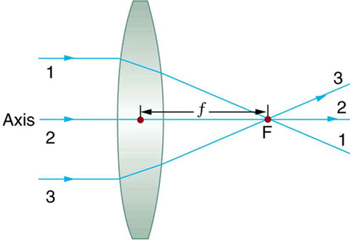
• A convex lens collect, or focus, parallel rays into a single focus point.
• This works as a burning glass.
  • The sun is so far away that the sun rays are parallel for all practical purposes.
• Definitions
  • Optical Axis is the line perpendicular on the lens, through its centre.
  • The Focus is a point on the Optical Axis. Rays which enter the lense parallel to the optical axis are deflected so that they intersect at the Focus.
  • Focal Length is the distance between the lens and the Focus. (We ignore the thickness of the lens.)
  • The Focal Plane is a plane through the Focus, perpendicular on the Optical Axis.

The Image Plane

• The image plane
  • non-parallel rays
• The thin lens equation
• Points further away
• The aperture

The pinhole model

• Reference frame
• Co-ordinates

Geometry of Image Formation

Exercises

Debrief

Credits

Introduction to Psychology by University of Minnesota is licensed under a Creative Commons Attribution-NonCommercial-ShareAlike 4.0 International License, except where otherwise noted.

College Physics. Authored by: OpenStax College. License: CC BY: Attribution. License Terms: Located at License