Reading Ma 2004 Chapters 5 and 3.3.4

Goal Reconstruct 3D points from stereo vision by triangulation.

Main Features

1. Triangulation allows us to calculate the depth of a point in 3D using the relative pose, i.e. the co-ordinate transform \((R,T)\) between the two camera frames.
2. The Essential Matrix describes the relationship between the two camera frames.
3. In the next session we will
   1. Use the eight point algorithm to find the essential matrix
   2. Decompose the Essential Matrix to get the co-ordinate transformation \((R,T)\) between the camera frames.

(1) Relative Pose

• Two cameras, two co-ordinate frames
• Relative Pose: transformation \((R,T)\) from Camera Frame 1 to Camera Frame 2.
• Consider a point \(p\) in 3D, it has
  • co-ordinates \(\mathbf{X}_i\) in Camera Frame \(i\)
• The projection of \(\mathbf{X}_i\) in homogeneous co-ordinates is called \(\mathbf{x}_i\)
  • \(\mathbf{X}_i = \lambda_i\mathbf{x}_i\)
  • Note \(\mathbf{x}_i\) is 3D co-ordinates if the image plane is normalised to \(z=1\)
• Combining this with the relation \(\mathbf{X}_2=R\mathbf{X}_1+T\), we get \[\lambda_2\mathbf{x}_2 = R\lambda_1\mathbf{x}_1 + T\]

(2) The Epipolar Constraint

• The epipolar plane \(P\) is spanned by \(T\) and \(p\)
• Multiply by \(\hat T\) to get a vector orthogonal on \(P\) \[\lambda_2\hat T\mathbf{x}_2 = \hat TR\lambda_1\mathbf{x}_1 + \hat TT\]
• The last term is zero because \(T\times T=0\) \[\lambda_2\hat T\mathbf{x}_2 = \hat TR\lambda_1\mathbf{x}_1\]
• Now \(\mathbf{x}_2\) is perpendicular on \(T\times\mathbf{X}_2\) so \[0=\mathbf{x}_2^T\lambda_2\hat T\mathbf{x}_2 = \mathbf{x}_2^T\hat TR\lambda_1\mathbf{x}_1\]
• Since \(\lambda_1\) is a scalar, we can simplify \[0= \mathbf{x}_2^T\hat TR\mathbf{x}_1\] This is the epipolar constraint
• \(E=\hat TR\) is called the essential matrix
  • We will use this later in the Eight-point algorithm

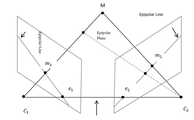
Epipolar Entities

• For each point \(p\), we have
  • a epipolar plane \(\langle o_1,o_2,p\rangle\)
  • epipolar line \(\ell_i\) as the intersection of the epipolar plane and the image plane
• The epipoles \(\mathbf{e}_i\) is the projection of origo onto the image plane of the other camera.
• Note that the epipoles are on the line \(\langle o_1,o_2\rangle\), and hence in the epipolar plane

Some properties

Proposition 5.3(1)

\[\mathbf{e}_2^TE = E\mathbf{e}_1=0\]

• This is because
  1. \(\mathbf{e}_2\sim T\) and \(\mathbf{e}_1\sim R^TT\)
  2. \(E=\hat TR\)
  3. \(T\hat T = T\times T=0\)

Proposition 5.3(2)

Proposition 5.3(3)

• Both the image point and the epipole lie on the epipolar line

(3) Pre- and Co-Image

Projections from 3D to 2D

• Recall that each point \(x\) in the image plane is the image of any point on a line through \(O\)
  • Correspondence between lines through \(O\) and point in the image.
  • This line is called the pre-image of \(x\).

Draw frontal model with image at \(Z=1\). This gives projective image co-ordinage \((x,y,1)\) embedded in 3D.

• What about a line \(l\) in the image plane? What is the pre-image?
  • Plane \(P\) through the origin. The line \(l\) is the intersection of \(P\) and the image plane
• What is the image of a line \(L\) in 3D?
  • if \(O\in L\) we have a point, whose pre-image is \(L\)
  • if \(O\not\in L\), we have a line \(l\) whose pre-image is a plane \(P\ni O\)
  • \(P\) is described by an orthogonal vector, the dual space \(P^\bot\),
    which we call the co-image of \(l\)

Linear objects in 2D

• The most important linear object is the line through the origin.
  • These are subspaces of dimension one.
• The object is a set \(\ell\subset\mathbb{R}^2\)
• Three descriptions
  • functions \[\ell = \{ \vec{x}=(x,y) | y = a\cdot x, x\in\mathbb{R} \}\] for some \(a\in\mathbb{R}\)
    • Exception: The vertical line would have \(a=\infty\), for infinitely steep
  • equations \[\ell = \{ \vec{x}=(x,y) | \vec{x}\cdot\vec{x}^\bot \}\] for some \(\vec{x}^\bot\in\mathbb{R}^2\)
    • Note that for \(c\neq0\), \(\vec{x}^\bot\) and \(c\vec{x}^\bot\) define the same line.
  • span \[\ell = \{ \vec{x}=(x,y) | a\cdot \vec{x}_0, a\in\mathbb{R} \}\] for some \(\vec{x}_0\in\mathbb{R}^2\)
    • Exception: The vertical line would have \(a=\infty\), for infinitely steep

If we normalise \(\vec{x}^\bot\), we can write \(\vec{x}^\bot=(a,1)\) for \(a\in\mathbb{R}\) unless we describe the vertical line, which has \(\vec{x}^\bot=(1,0)\), which we could imagine writing \((\infty,1)\).

• We can normalise \(\vec{x}_0\) in the same way.
• The set of lines through origo is equivalent to \(\mathbb{R}\cup\{\infty\}\), which can be seen in either representation.

Linear objects in 3D

We have the same situation in 3D, but we have more objects of interest.

• In 2D, the line is defined by one function or one equation.
• In 3D we have
  • the line \(\ell= \{(x,y,z) | z = ax + by, (x,y)\in\mathbb{R}\}\)
  • the plane \(\mathcal{P}= \{(x,y,z) | z = ax, y = bx, x\in\mathbb{R}^2\}\) (two function)
• Using equations to define it
  • The plane needs one equation \[\mathcal{P}=\{\vec{x} | \vec{x}\cdot\vec{x}^\bot=0 \}\]
    • \(\vec{x}^\bot\) is the dual space \(\mathcal{P}\)
  • The line needs two equation \[\ell=\{\vec{x} | \vec{x}\cdot\vec{y}_1=0, \vec{x}\cdot\vec{y}_1=0\}\]
    • The space spanned by \(\vec{y}_1\) and \(\vec{y}_2\) is the dual space \(\ell^\bot\)
• What does it look like as spans?
• An object needs
  • one function per dimension; or
    • Each adds one degree of freedom
  • one equation per codimension
    • Each equation removes one degree of freedom

Projections from 3D to 2D

• Recall that each point \(x\) in the image plane is the image of any point on a line through \(O\)
  • Correspondence between lines through \(O\) and point in the image.
  • This line is called the pre-image of \(x\).

Draw frontal model with image at \(Z=1\). This gives projective image co-ordinage \((x,y,1)\) embedded in 3D.

• What about a line \(l\) in the image plane? What is the pre-image?
  • Plane \(P\) through the origin. The line \(l\) is the intersection of \(P\) and the image plane
• What is the image of a line \(L\) in 3D?
  • if \(O\in L\) we have a point, whose pre-image is \(L\)
  • if \(O\not\in L\), we have a line \(l\) whose pre-image is a plane \(P\ni O\)
  • \(P\) is described by an orthogonal vector, the dual space \(P^\bot\),
    which we call the co-image of \(l\)

Epipolar Geometry

When the textbook defines the epipolar line as the null space of \(\hat TR\mathrm{x}_1\), this is a simplification. The null space is the epipolar plane, and the epipolar line is only those points that also fall in the image plane. Two equations are needed to define the epipolar line in 3D:

1. \(x^TEx_1=T\times Rx_1\)
2. \(x^T[0,0,1]^T=1\) (i.e. \(z=1\))

When we say that \(\ell_2\sim Ex_1\), it is abuse of terminology. It is the co-image of \(\ell_2\) of \(Ex_1\). The actual line (set of points) is those points that are orthogonal on \(Ex_1\). This is not a problem when we are aware of the abuse.

Note that we work on 3D points all the way. We have not defined an origin in the image plane, and trying to see why \(x_2\) and \(Ex_1\) be orthogonal as 2D vectors is not helpful.

(4) Triangulation

Question How do we find \(\lambda\) when \((R,T)\) is known?

1. We can find the angle between image point \(x\) and epipole \(e\) \[\cos\theta = \frac{x\cdot e}{||x||\cdot||e||}\]
2. We can reconstruct \(\lambda\) using the sine law \[ \frac{\sin\theta_{\mathrm{II}}}{\lambda_2}= \frac{\sin\theta_{\mathrm{I}}}{\lambda_1} = \frac{\sin\theta_{0}}{||T||}\]
3. It is also possible to use the cosine law

See PDF figure

(5) Finding the Relative Pose

The rest of this document is a teaser for sessions to come.

Decomposition of the Essential Matix

• Theorem 5.5

\[E = U\mathsf{diag}\{\sigma,\sigma,0\}V^T,\] where \(U,V\in\mathsf{SO}(3)\)

• Tricky proof. Do not spend too much time on this.

\[ \begin{cases} (\hat T_1,R_1) &= (UR_Z(+\frac\pi2)\Sigma U^T, UR_Z(+\frac\pi2)V^T) \\ (\hat T_2,R_2) &= (UR_Z(-\frac\pi2)\Sigma U^T, UR_Z(-\frac\pi2)V^T) \end{cases} \] where \[R_Z(+\frac\pi2) = \begin{bmatrix} 0 & -1 & 0 \\ 1 & 0 & 0 \\ 0 & 0 & 1 \end{bmatrix} \] is a rotation by \(\pi/2\) radians around the \(z\)-axis.

• Note that there are two solutions from one \(U\Sigma V^T\) decomposition.
• Are there more solutions?

Two Relative Poses

There exist exactly two relative poses \((R,T)\) with \(R\in\mathsf{SO}(3)\) and \(T\in\mathbb{R}^3\) corresponding to a nonzero essential matrix \(E\in\mathcal{E}\) Theorem 5.7

Repetition

• Rotation by angle \(\theta\) around the vector \(\omega\) is given by \(R=e^{\hat\omega\theta}\) assuming \(\omega\) has unit length.

Rodrigues’ formula (2.16)

\[e^{\hat\omega} = I + \frac{\hat\omega}{||\omega||}\sin(||\omega||) + \frac{\hat\omega^2}{||\omega||^2}(1-\cos(||\omega||))\]

See Angular Motion for a more comprehensive summary.

Theorem 5.7

• Demo read the proof (debrief?)

Lemma 5.6

If \(\hat T\) and \(\hat TR\) are both skew-symmetric for \(R\in\mathrm{SO}(3)\), then \(R\) is a rotation by angle \(\pi\) around \(T\).

• Demo read the proof (debrief?)

• Skew-symmetry gives \((\hat TR)^T=-\hat TR\)
• We also have \((\hat TR)^T=R^T\hat T^T=-R^T\hat T\)
• Hence \(\hat TR = R^T\hat T\),
• and since \(R^T=R^{-1}\), we have \[R\hat TR=\hat T\]
• Write \(R=e^{\hat\omega\theta}\) for some \(\omega\) of unit length and some \(\theta\), to get \[e^{\hat\omega\theta}\hat Te^{\hat\omega\theta}=\hat T\]

• multiply by \(\omega\) \[e^{\hat\omega\theta}\hat Te^{\hat\omega\theta}\omega=\hat T\omega\] This represents a stationary rotation of the vector \(\hat T\omega\).

Note that \(\omega\) is stationary under rotation by \(R\), and hence it is an eigenvector associated with eigenvalue 1. Furthermore, it is the only such eigenvector, and \(\hat T\omega\) cannot be such. Hence \(\hat T\omega=T\times\omega=0\). This is only possible if \(T\sim\omega\), and since \(\omega\) has unit length, we get \[\omega = \pm\frac{T}{||T||}\]

We now know that \(R\) has to be a rotation around \(T\), and therefore \(R\) and \(T\) commute. This can be checked in Rodrigues’ formula (Theorem 2.9).

Hence \(R^2\hat T = \hat T\). This looks like two half-round rotations to get back to start. If \(\hat T\) had been a vector or a matrix of full rank, we would have been done. However, with the skew-symmetric \(\hat T\) there is a little more fiddling.