Reading Ma 2004 Chapter 5

The Epipolar Constraint

• Two cameras, two co-ordinate frames
• Relative Pose: transformation \((R,T)\) from Camera Frame 1 to Camera Frame 2.
• Consider a point \(p\) in 3D, it has
  • co-ordinates \(\mathbf{X}_i\) in Camera Frame \(i\)
• The projection of \(\mathbf{X}_i\) in homogeneous co-ordinates is called \(\mathbf{x}_i\)
  • \(\mathbf{X}_i = \lambda_i\mathbf{x}_i\)
  • Note \(\mathbf{x}_i\) is 3D co-ordinates if the image plane is normalised to \(z=1\)
• Combining this with the relation \(\mathbf{X}_2=R\mathbf{X}_1+T\), we get \[\lambda_2\mathbf{x}_2 = R\lambda_1\mathbf{x}_1 + T\]
• To simplify, we multiply by \(\hat T\) to get \[\lambda_2\hat T\mathbf{x}_2 = \hat TR\lambda_1\mathbf{x}_1 + \hat TT\]
• The last term is zero because \(T\times T=0\) \[\lambda_2\hat T\mathbf{x}_2 = \hat TR\lambda_1\mathbf{x}_1\]
• Now \(\mathbf{x}_2\) is perpendicular on \(T\times\mathbf{X}_2\) so \[0=\mathbf{x}_2^T\lambda_2\hat T\mathbf{x}_2} = \mathbf{x}_2^T\hat TR\lambda_1\mathbf{x}_1\]
• Since \(\lambda_1\) is a scalar, we can simplify \[0= \mathbf{x}_2^T\hat TR\mathbf{x}_1\] This is the epipolar constraint
• \(E=\hat TR\) is called the essential matrix

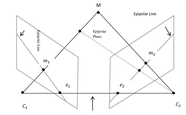
Some Jargon

• For each point \(p\), we have
  • a epipolar plane \(\langle o_1,o_2,p\rangle\)
  • epipolar line \(\ell_i\) as the intersection of the epipolar plane and the image plane
• The epipoles \(\mathbf{e}_i\) is the projection of origo onto the image plane of the other camera.
• Note that the epipoles are on the line \(\langle o_1,o_2\rangle\), and hence in the epipolar plane

Some properties

Proposition 5.3(1)

\[\mathbf{e}_2^TE = E\mathbf{e}_1=0\]

• This is because
  1. \(\mathbf{e}_2\sim T\) and \(\mathbf{e}_1\sim R^TT\)
  2. \(E=\hat TR\)
  3. \(T\hat T = T\times T=0\)

Proposition 5.3(2)

Proposition 5.3(3)

• Both the image point and the epipole lie on the epipolar line

Eight-Point Algorithm

\[\mathbf{x}_2^TE\mathbf{x}_1 = 0\]

Kronecker product: \(\bigotimes\)

Serialisation of a matrix: \((\cdot)^\)

\[(\mathbf{x}_1\bigotimes\mathbf{x}_2)^TE^s = 0\]

\[\mathbf{a} = \mathbf{x}_1\bigotimes\mathbf{x}_2\]

\[\chi = [mathbf{a}_1, mathbf{a}_2, \ldots, mathbf{a}_n]\]

We can solve \(\chiE^s = 0\) for \(E^s\). With eight points, we have unique solutions up to a scalar factor.

The solution is not necessarily a valid essential matrix, but we can project onto the space of such matrices and correct the sign to get positive determinant.