Reading Ma 2004 Chapter 5

The Epipolar Constraint

• Two cameras, two co-ordinate frames
• Relative Pose: transformation \((R,T)\) from Camera Frame 1 to Camera Frame 2.
• Consider a point \(p\) in 3D, it has
  • co-ordinates \(\mathbf{X}_i\) in Camera Frame \(i\)
• The projection of \(\mathbf{X}_i\) in homogeneous co-ordinates is called \(\mathbf{x}_i\)
  • \(\mathbf{X}_i = \lambda_i\mathbf{x}_i\)
  • Note \(\mathbf{x}_i\) is 3D co-ordinates if the image plane is normalised to \(z=1\)
• Combining this with the relation \(\mathbf{X}_2=R\mathbf{X}_1+T\), we get \[\lambda_2\mathbf{x}_2 = R\lambda_1\mathbf{x}_1 + T\]
• To simplify, we multiply by \(\hat T\) to get \[\lambda_2\hat T\mathbf{x}_2 = \hat TR\lambda_1\mathbf{x}_1 + \hat TT\]
• The last term is zero because \(T\times T=0\) \[\lambda_2\hat T\mathbf{x}_2 = \hat TR\lambda_1\mathbf{x}_1\]
• Now \(\mathbf{x}_2\) is perpendicular on \(T\times\mathbf{X}_2\) so \[0=\mathbf{x}_2^T\lambda_2\hat T\mathbf{x}_2 = \mathbf{x}_2^T\hat TR\lambda_1\mathbf{x}_1\]
• Since \(\lambda_1\) is a scalar, we can simplify \[0= \mathbf{x}_2^T\hat TR\mathbf{x}_1\] This is the epipolar constraint
• \(E=\hat TR\) is called the essential matrix

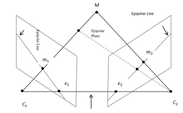
Epipolar Entities

• For each point \(p\), we have
  • a epipolar plane \(\langle o_1,o_2,p\rangle\)
  • epipolar line \(\ell_i\) as the intersection of the epipolar plane and the image plane
• The epipoles \(\mathbf{e}_i\) is the projection of origo onto the image plane of the other camera.
• Note that the epipoles are on the line \(\langle o_1,o_2\rangle\), and hence in the epipolar plane

Some properties

Proposition 5.3(1)

\[\mathbf{e}_2^TE = E\mathbf{e}_1=0\]

• This is because
  1. \(\mathbf{e}_2\sim T\) and \(\mathbf{e}_1\sim R^TT\)
  2. \(E=\hat TR\)
  3. \(T\hat T = T\times T=0\)

Proposition 5.3(2)

Proposition 5.3(3)

• Both the image point and the epipole lie on the epipolar line

Decomposition of the Essential Matix

• Theorem 5.5

Two Relative Poses

• Theorem 5.7

Repetition

• Rotation by angle \(\theta\) around the vector \(\omega\) is given by \(R=e^{\hat\omega\theta}\) assuming \(\omega\) has unit length.

Rodrigues’ formula (2.16)

\[e^{\hat\omega} = I + \frac{\hat\omega}{||\omega||}\sin(||\omega||) + \frac{\hat\omega^2}{||\omega||^2}(1-\cos(||\omega||))\]

Lemma 5.6

If \(\hat T\) and \(\hat TR\) are both skew-symmetric for \(R\in\mathrm{SO}(3)\), then \(R\) is a rotation by angle \(\pi\) around \(T\).

• Skew-symmetry gives \((\hat TR)^T=-\hat TR\)
• We also have \((\hat TR)^T=R^T\hat T^T=-R^T\hat T\)
• Hence \(\hat TR = R^T\hat T\),
• and since \(R^T=R^{-1}\), we have \[R\hat TR=\hat T\]
• Write \(R=e^{\hat\omega\theta}\) for some \(\omega\) of unit length and some \(\theta\), to get \[e^{\hat\omega\theta}\hat Te^{\hat\omega\theta}=\hat T\]
• multiply by \(\omega\) \[e^{\hat\omega\theta}\hat Te^{\hat\omega\theta}\omega=\hat T\omega\] This represents a stationary rotation of the vector \(\hat T\omega\).

Note that \(\omega\) is stationary under rotation by \(R\), and hence it is an eigenvector associated with eigenvalue 1. Furthermore, it is the only such eigenvector, and \(\hat T\omega\) cannot be such. Hence \(\hat T\omega=T\times\omega=0\). This is only possible if \(T\sim\omega\), and since \(\omega\) has unit length, we get \[\omega = \pm\frac{T}{||T||}\]

We now know that \(R\) has to be a rotation around \(T\), and therefore \(R\) and \(T\) commute. This can be checked in Rodrigues’ formula (Theorem 2.9).

Hence \(R^2\hat T = \hat T\). This looks like two half-round rotations to get back to start. If \(\hat T\) had been a vector or a matrix of full rank, we would have been done. However, with the skew-symmetric \(\hat T\) there is a little more fiddling.